Scraping Autotrader Data with R
Car Economics
About a month ago I was looking at buying a car and considering that if I could understand the average price of any model at 200k miles--relative to it's sale price--then I could gauge the quality of the car and infer its probability of costly repairs into the later stages of its useful life.
I also knew, anectodally, that a car depreciates most rapidly in it's initial years then more slowly as time goes on (i.e. it is not a straight line depreciation situation); and I wanted to quantify that with real data then use the data to help me decide what the most economic decision would be in terms of the net present value of all related future cashflows for a car purchase made now extending over a 10-year period. So, what point along the car's lifecyle is the optimum time to buy?
I was doing a lot of Auto Trader searches at the time and learned there was no publicly available API to access the UK data. What follows is instructions on how to scrape autotrader search results from the website (note: the below works for autotrader.co.uk, but a similar approach may also work for other country sites).
The Final Solution (R Code)
###############################################################################
##                        Scraping AutoTrader Data
###############################################################################
#This code scrapes car advertising data from various Auto Trader search queries
#
#Inputs:
#   - Autotrader website (uk)
#
#Anatomy:
# 1. Set Up
# 2. Create Shell Dataframe
# 3. Srape Page Data
# 4. Output to Excel

##1. Set Up
#install rvest
install.packages('rvest')
#set working directory (cache)
setwd('C:/Users/craig/Google Drive/201706/0626cars_economics/cache')#change this to a path that exists on your computer
#reference rvest library
library(rvest)

##2. Create Shell Dataframe
df_base<-data.frame(model=character(),year=character(),miles=character(),
    gearshift=character(),engine_size=character(),location=character(),
    location=character())

##3. Scrape Page Data
#declare root url'
rooturl<-'http://www.autotrader.co.uk/car-search?sort=sponsored&radius=1500&postcode=ky119sb&onesearchad=Used&onesearchad=Nearly%20New&onesearchad=New&make=TOYOTA&model=VERSO&year-from=1990&year-to=2017&minimum-mileage=0&maximum-mileage=200000&body-type=MPV&fuel-type=Diesel&minimum-badge-engine-size=1.6&maximum-badge-engine-size=4.5&minimum-seats=7&maximum-seats=8&page='
#scrape the data
for (i in 1:34){
  #read html into R
  url_string<-paste(rooturl,i,sep='')
  tpage<-read_html(url_string)
  #create a dataframe with all the relevant nodes df1<-data.frame(model=html_text(html_nodes(tpage,'.listing-title.title-wrap')),
      year=html_text(html_nodes(tpage,'.listing-key-specs li:nth-child(1)')),
      miles=html_text(html_nodes(tpage,'.listing-key-specs li:nth-child(3)')),
      gearshift=html_text(html_nodes(tpage,'.listing-key-specs li:nth-child(4)')),
      engine_size=html_text(html_nodes(tpage,'.listing-key-specs li:nth-child(5)')),
      location=html_text(html_nodes(tpage,'.seller-location')),
      price=html_text(html_nodes(tpage,'.vehicle-price'))
  )
  #append the data to df_base (shell dataframe)
  df_base<-rbind(df_base,df1)
}

##4. output to excel
#check dimentions
dim(df_base)
#output as .csv for inspection
write.csv(df_base,'versos.csv')
If you paste the above code snippet into R Studio and run it, then you should see some results dropping into a spreadsheet in your working directory for Toyota Versos (note that you would need to change your working directory to a path that exists on your machine first!) However, you most likely will want to know how the code was devised so you can apply the principles to other potential searches. So I will walk you through the process of how to customise the above solution to your needs.
1. The Website
It is worth starting with the actual website. Go to Autotrader.co.uk and type in some search criteria for any type of car you are after. If I type in some criteria for Versos, for example, it takes me to a page that looks like this:
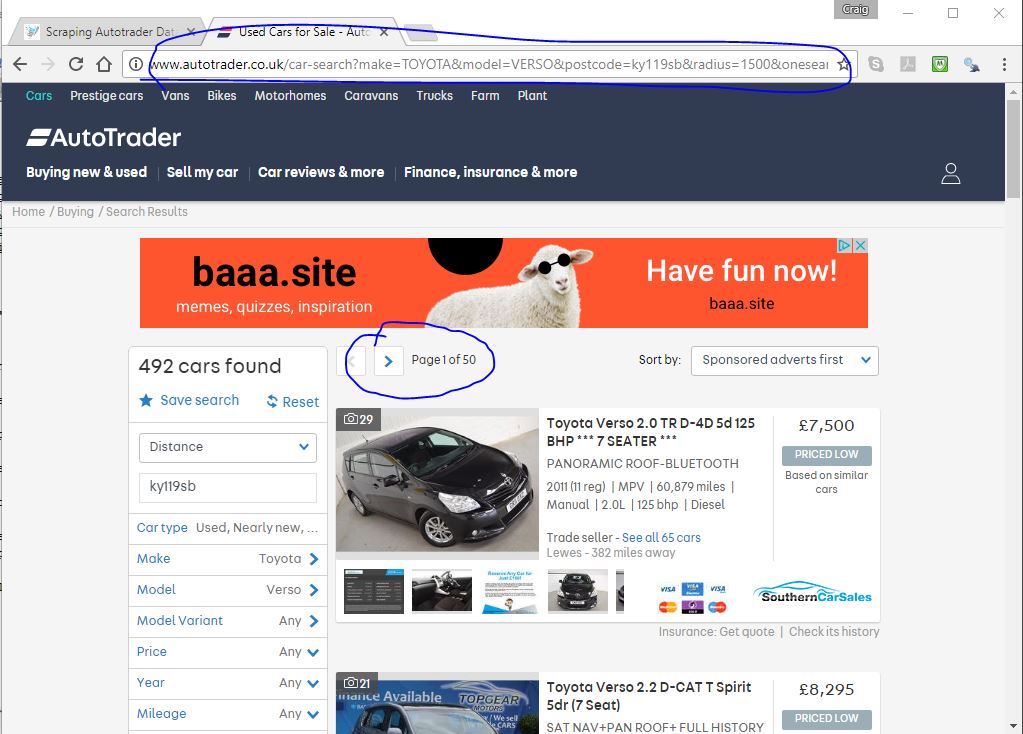
There are three things to note here: (1) the web address contains a reference to a url made up of all your search criteria, (2) notice that when you click on the arrow icon next to where it says 'Page 1 of 50' on the webpage, the address updates slightly and adds 'page=2' on the end of the url, (3) the page is essentially made up of 10 cars with a picture, then some information next to the picture--like a list. What we are going to do is find tags or classes that your browser uses to classify or format the bits of information that are of interest.
2. SelectorGadget
I'm using Chrome and if I right-click on any item on the page I get a drop-down menu from which I can then select 'inspect code' to look at which html and css tags are associated with the item. You can figure out the associated tags for the data you need this way, but it can be quite difficult to get it right and what tends to happen is that you think you are selecting the correct identifying tags only to later find that you have selected unwanted items in addition to the ones you need. This is where SelectorGadget becomes extremely useful. To use it just use the above link and, as stated there, drag it into your bookmarks bar.
At this point I would refer you to Hadley Wickham's excellent brief rvest webscraping tutorial for a really easy to follow tutorial on extracting imdb data on The Lego Movie. Hadley also references selectorgadget in that tutorial. It will not yet be clear why you need to gather the correct tag locators; however, after we look at RVEST and some R code, you will see the relevance.
3. RVEST in R
Assuming you have R Studio installed (if you haven't then brief instructions to do so are in my house price machine learning article. It is pretty quick and easy to do), install the RVEST package wit install.packages('rvest') as shown in the snippet above then reference the rvest library (also shown above). Make sure you set the working directory (setwd) to a valid path on your computer.
Next, ignore all the other code from the above snippet and focus on the below part only (copied from above):
df1<-data.frame(model=html_text(html_nodes(tpage,'.listing-title.title-wrap')),
      year=html_text(html_nodes(tpage,'.listing-key-specs li:nth-child(1)')),
      miles=html_text(html_nodes(tpage,'.listing-key-specs li:nth-child(3)')),
      gearshift=html_text(html_nodes(tpage,'.listing-key-specs li:nth-child(4)')),
      engine_size=html_text(html_nodes(tpage,'.listing-key-specs li:nth-child(5)')),
      location=html_text(html_nodes(tpage,'.seller-location')),
      price=html_text(html_nodes(tpage,'.vehicle-price'))
  )
In fact, just look at the first line of that section that starts 'df1<-'. What the code is doing here is creating a new dataframe called df1 that contains all the relevant parsed items from one html page. Look back at the complete code and see that tpage is actually created from 'read_html(url_string)' which basically means tpage is all the html code from one url. The url_string the url of the search results page we saw above with i added to the end... which we will just say is 1 for now. So the code is looking at the html code for the page and using the rvest's html_text() and html_nodes() functions to extract a list of all the relevant nodes into one column per node type.
For example, taking the first column in our df1 dataframe... this has been assigned the label 'model' and it is equal to a list of all html nodes with the selector tags matching '.listing-title.title-wrap'. The result is the first column of our dataframe being named 'model and containing all the model fields from the webpage.
The second column, similarly looks for all html nodes with the selector tag '.listing-key-specs li:nth-child(1)'... which we have mined using the SelectorGadget tool and understand to be 'year', i.e. year the car was manufactured.
Through a similar process all other desired characteristics (miles, gearshift, engine_size, location, and price) have been collated into the df1 dataframe. And this is essentially the guts of the exercise. If you have managed to get this far you are 95% there. The tricky part is identifying the correct selector tags--but SelectorGadget is a tremendous help when it comes to this.
4. Wrapping it Up
As mentioned above, each page in the search results is indexed from 1 to however many pages your search returns. I the case of the code above, it was 34 pages. And so, the code has been written to create an empty base dataframe then repeat the dataframe creation step 34 times--once for each url in the sequence of search result pages--each time appending the newly created dataframe to base dataframe.
The last step in the above code snippet is to write the resulting dataframe to a csv file for analysis. Note that for the above process to work each field must be populated in every result generated. To ensure this I had to complete min and max range options on every search criterion on the Autotrader website. I also tried to perform the scrape for queries with over 100 returned pages. But the website limits results at 100 pages. So if a set of results with >100 pages is needed they would need to be processed in batches.